Time series analysis
Cloud services and IoT devices generate telemetry data that can be used to gain insights such as monitoring service health, physical production processes, and usage trends. Performing time series analysis is one way to identify deviations in the pattern of these metrics compared to their typical baseline pattern.
Kusto Query Language (KQL) contains native support for creation, manipulation, and analysis of multiple time series. In this article, learn how KQL is used to create and analyze thousands of time series in seconds, enabling near real-time monitoring solutions and workflows.
Time series creation
In this section, we'll create a large set of regular time series simply and intuitively using the make-series operator, and fill-in missing values as needed.
The first step in time series analysis is to partition and transform the original telemetry table to a set of time series. The table usually contains a timestamp column, contextual dimensions, and optional metrics. The dimensions are used to partition the data. The goal is to create thousands of time series per partition at regular time intervals.
The input table demo_make_series1 contains 600K records of arbitrary web service traffic. Use the following command to sample 10 records:
demo_make_series1 | take 10
The resulting table contains a timestamp column, three contextual dimensions columns, and no metrics:
| TimeStamp | BrowserVer | OsVer | Country/Region |
|---|---|---|---|
| 2016-08-25 09:12:35.4020000 | Chrome 51.0 | Windows 7 | United Kingdom |
| 2016-08-25 09:12:41.1120000 | Chrome 52.0 | Windows 10 | |
| 2016-08-25 09:12:46.2300000 | Chrome 52.0 | Windows 7 | United Kingdom |
| 2016-08-25 09:12:46.5100000 | Chrome 52.0 | Windows 10 | United Kingdom |
| 2016-08-25 09:12:46.5570000 | Chrome 52.0 | Windows 10 | Republic of Lithuania |
| 2016-08-25 09:12:47.0470000 | Chrome 52.0 | Windows 8.1 | India |
| 2016-08-25 09:12:51.3600000 | Chrome 52.0 | Windows 10 | United Kingdom |
| 2016-08-25 09:12:51.6930000 | Chrome 52.0 | Windows 7 | Netherlands |
| 2016-08-25 09:12:56.4240000 | Chrome 52.0 | Windows 10 | United Kingdom |
| 2016-08-25 09:13:08.7230000 | Chrome 52.0 | Windows 10 | India |
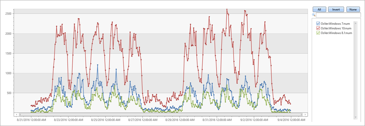
Since there are no metrics, we can only build a set of time series representing the traffic count itself, partitioned by OS using the following query:
let min_t = toscalar(demo_make_series1 | summarize min(TimeStamp));
let max_t = toscalar(demo_make_series1 | summarize max(TimeStamp));
demo_make_series1
| make-series num=count() default=0 on TimeStamp from min_t to max_t step 1h by OsVer
| render timechart
- Use the
make-seriesoperator to create a set of three time series, where:num=count(): time series of trafficfrom min_t to max_t step 1h: time series is created in 1-hour bins in the time range (oldest and newest timestamps of table records)default=0: specify fill method for missing bins to create regular time series. Alternatively useseries_fill_const(),series_fill_forward(),series_fill_backward()andseries_fill_linear()for changesby OsVer: partition by OS
- The actual time series data structure is a numeric array of the aggregated value per each time bin. We use
render timechartfor visualization.
In the table above, we have three partitions. We can create a separate time series: Windows 10 (red), 7 (blue) and 8.1 (green) for each OS version as seen in the graph:

Time series analysis functions
In this section, we'll perform typical series processing functions. Once a set of time series is created, KQL supports a growing list of functions to process and analyze them. We'll describe a few representative functions for processing and analyzing time series.
Filtering
Filtering is a common practice in signal processing and useful for time series processing tasks (for example, smooth a noisy signal, change detection).
- There are two generic filtering functions:
series_fir(): Applying FIR filter. Used for simple calculation of moving average and differentiation of the time series for change detection.series_iir(): Applying IIR filter. Used for exponential smoothing and cumulative sum.
Extendthe time series set by adding a new moving average series of size 5 bins (named ma_num) to the query:
let min_t = toscalar(demo_make_series1 | summarize min(TimeStamp));
let max_t = toscalar(demo_make_series1 | summarize max(TimeStamp));
demo_make_series1
| make-series num=count() default=0 on TimeStamp from min_t to max_t step 1h by OsVer
| extend ma_num=series_fir(num, repeat(1, 5), true, true)
| render timechart

Regression analysis
Azure Data Explorer supports segmented linear regression analysis to estimate the trend of the time series.
- Use series_fit_line() to fit the best line to a time series for general trend detection.
- Use series_fit_2lines() to detect trend changes, relative to the baseline, that are useful in monitoring scenarios.
Example of series_fit_line() and series_fit_2lines() functions in a time series query:
demo_series2
| extend series_fit_2lines(y), series_fit_line(y)
| render linechart with(xcolumn=x)

- Blue: original time series
- Green: fitted line
- Red: two fitted lines
Note
The function accurately detected the jump (level change) point.
Seasonality detection
Many metrics follow seasonal (periodic) patterns. User traffic of cloud services usually contains daily and weekly patterns that are highest around the middle of the business day and lowest at night and over the weekend. IoT sensors measure in periodic intervals. Physical measurements such as temperature, pressure, or humidity may also show seasonal behavior.
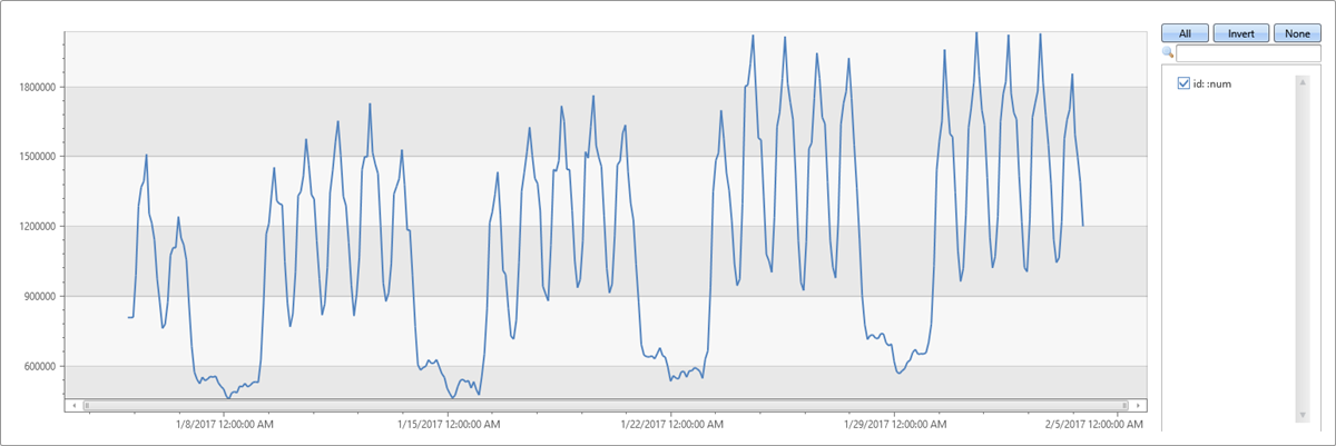
The following example applies seasonality detection on one month traffic of a web service (2-hour bins):
demo_series3
| render timechart

- Use series_periods_detect() to automatically detect the periods in the time series.
- Use series_periods_validate() if we know that a metric should have specific distinct period(s) and we want to verify that they exist.
Note
It's an anomaly if specific distinct periods don't exist
demo_series3
| project (periods, scores) = series_periods_detect(num, 0., 14d/2h, 2) //to detect the periods in the time series
| mv-expand periods, scores
| extend days=2h*todouble(periods)/1d
| periods | scores | days |
|---|---|---|
| 84 | 0.820622786055595 | 7 |
| 12 | 0.764601405803502 | 1 |
The function detects daily and weekly seasonality. The daily scores less than the weekly because weekend days are different from weekdays.
Element-wise functions
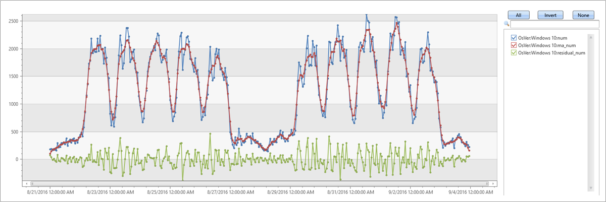
Arithmetic and logical operations can be done on a time series. Using series_subtract() we can calculate a residual time series, that is, the difference between original raw metric and a smoothed one, and look for anomalies in the residual signal:
let min_t = toscalar(demo_make_series1 | summarize min(TimeStamp));
let max_t = toscalar(demo_make_series1 | summarize max(TimeStamp));
demo_make_series1
| make-series num=count() default=0 on TimeStamp in from min_t to max_t step 1h by OsVer
| extend ma_num=series_fir(num, repeat(1, 5), true, true)
| extend residual_num=series_subtract(num, ma_num) //to calculate residual time series
| where OsVer == "Windows 10"   // filter on Win 10 to visualize a cleaner chart
| render timechart

- Blue: original time series
- Red: smoothed time series
- Green: residual time series
Time series workflow at scale
The example below shows how these functions can run at scale on thousands of time series in seconds for anomaly detection. To see a few sample telemetry records of a DB service's read count metric over four days run the following query:
demo_many_series1
| take 4
| TIMESTAMP | Loc | Op | DB | DataRead |
|---|---|---|---|---|
| 2016-09-11 21:00:00.0000000 | Loc 9 | 5117853934049630089 | 262 | 0 |
| 2016-09-11 21:00:00.0000000 | Loc 9 | 5117853934049630089 | 241 | 0 |
| 2016-09-11 21:00:00.0000000 | Loc 9 | -865998331941149874 | 262 | 279862 |
| 2016-09-11 21:00:00.0000000 | Loc 9 | 371921734563783410 | 255 | 0 |
And simple statistics:
demo_many_series1
| summarize num=count(), min_t=min(TIMESTAMP), max_t=max(TIMESTAMP)
| num | min_t | max_t |
|---|---|---|
| 2177472 | 2016-09-08 00:00:00.0000000 | 2016-09-11 23:00:00.0000000 |
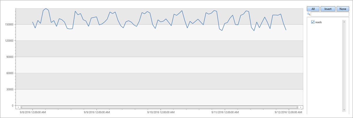
Building a time series in 1-hour bins of the read metric (total four days * 24 hours = 96 points), results in normal pattern fluctuation:
let min_t = toscalar(demo_many_series1 | summarize min(TIMESTAMP));
let max_t = toscalar(demo_many_series1 | summarize max(TIMESTAMP));
demo_many_series1
| make-series reads=avg(DataRead) on TIMESTAMP from min_t to max_t step 1h
| render timechart with(ymin=0)

The above behavior is misleading, since the single normal time series is aggregated from thousands of different instances that may have abnormal patterns. Therefore, we create a time series per instance. An instance is defined by Loc (location), Op (operation), and DB (specific machine).
How many time series can we create?
demo_many_series1
| summarize by Loc, Op, DB
| count
| Count |
|---|
| 18339 |
Now, we're going to create a set of 18339 time series of the read count metric. We add the by clause to the make-series statement, apply linear regression, and select the top two time series that had the most significant decreasing trend:
let min_t = toscalar(demo_many_series1 | summarize min(TIMESTAMP));
let max_t = toscalar(demo_many_series1 | summarize max(TIMESTAMP));
demo_many_series1
| make-series reads=avg(DataRead) on TIMESTAMP from min_t to max_t step 1h by Loc, Op, DB
| extend (rsquare, slope) = series_fit_line(reads)
| top 2 by slope asc
| render timechart with(title='Service Traffic Outage for 2 instances (out of 18339)')

Display the instances:
let min_t = toscalar(demo_many_series1 | summarize min(TIMESTAMP));
let max_t = toscalar(demo_many_series1 | summarize max(TIMESTAMP));
demo_many_series1
| make-series reads=avg(DataRead) on TIMESTAMP from min_t to max_t step 1h by Loc, Op, DB
| extend (rsquare, slope) = series_fit_line(reads)
| top 2 by slope asc
| project Loc, Op, DB, slope
| Loc | Op | DB | slope |
|---|---|---|---|
| Loc 15 | 37 | 1151 | -102743.910227889 |
| Loc 13 | 37 | 1249 | -86303.2334644601 |
In less than two minutes, close to 20,000 time series were analyzed and two abnormal time series in which the read count suddenly dropped were detected.
These advanced capabilities combined with fast performance supply a unique and powerful solution for time series analysis.
Related content
- Learn about Anomaly detection and forecasting with KQL.
- Learn about Machine learning capabilities with KQL.
Feedback
Coming soon: Throughout 2024 we will be phasing out GitHub Issues as the feedback mechanism for content and replacing it with a new feedback system. For more information see: https://aka.ms/ContentUserFeedback.
Submit and view feedback for